Before you get started, take note of these points:

• This guide discusses combining tables from the same workbook only, not external sources or multiple workbooks.
• Make sure all the datasets you want to append are formatted as Excel tables with column headers. Also, each table must contain the same column headers, though the columns don't have to be in the same order.
• For the process to work smoothly, check that each table is properly named according to the data it contains.

To follow along as you read this guide, download a free copy of the Excel workbook used in the example. After you click the link, you'll find the download button in the top right corner of your screen.

Step 1: Create Data Connections

Let's imagine you've been given an Excel workbook with two worksheets. The Vegetable_Prices_2022 worksheet contains a table named Vegetables, and the Fruit_Prices_2022 worksheet contains a table named Fruit.

Both tables contain the same column headers, though the columns are in a different order in each dataset. Your task is to stack the tables, one on top of the other, forming one dataset with all the information combined.

The first step involves creating connections between each of the datasets.

To do this, select any cell in the first table, and in the Data tab on the ribbon, click "From Table/Range."

Then, in the Power Query Editor, click the bottom half of the "Close And Load" button in the top-right corner, and select "Close And Load To."

Next, in the Import Data dialog box, select the "Only Create Connection" radio button, and click "OK."

At this point, the Queries And Connections pane opens on the right-hand side of the Excel window, where the connection you just created is listed.

Now, repeat this process for the remaining tables that you want to connect, and see them listed in the Queries And Connections pane as you go.

Step 2: Combine the Queries

Now that you've created the connections between the datasets, it's time to combine them physically.

In any worksheet in the workbook, head to the "Data" tab, click "Get Data," then select Combine Queries > Append.

Now, select the appropriate option according to the number of tables you're going to stack. In this case, you're stacking two datasets, so select "Two Tables." Then, use the drop-down menus to select the tables you want to append.

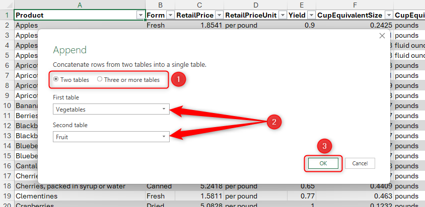
When you click "OK," the Power Query Editor reopens with the selected tables appended.

Notice how, even though the Form columns were in different places in each of the original datasets, the Power Query Editor recognized them as corresponding fields and merged them in the resultant append.

Step 3: Transform the Data in the Power Query Editor

Before you load the appended data back into your Excel workbook, make any necessary adjustments to the data's structure.

For example, because the two tables are still stacked, one on top of the other, you might want to sort the data by the Product column by clicking the filter button in the column header, and selecting "Sort Descending."

Second, it would make more sense to have the Form column next to the Product column, so click, drag, and drop it via the column header.

Finally, to make the product names stand out, right-click the column header, hover over "Transform," and click "Uppercase."

Step 4: Load the Newly Appended Data

Now that your data is appended and edited, you're ready to load it into your workbook.

Click the top half of the "Close And Load" button in the top-left corner of the Power Query Editor to load the table onto a new worksheet in the workbook.

For other options, like loading the data onto an existing worksheet or as a PivotTable, click the bottom half of the button, and select "Close And Load To."

Now, what were previously two datasets are neatly organized into one table.

If the source data changes, select any cell in the appended table, and in the Table Design tab, click "Refresh." This will ensure that the appended table always reflects the latest versions of the original data.

Additional Actions You Can Take

You don't have to stop there! Here are some other steps you can take to make the most of your newly generated data.

Adjust the Table's Properties

By default, tables generated through Power Query use the green medium 7 table style. To choose a different style, select any cell in the table, and select a style in the Table Style group of the Table Design tab on the ribbon.

While the Table Design tab is opened, review the selections in the Table Style Options group.

Append Another Table

If you want to append another table from a different worksheet to the existing append, first create a new connection by following step 1 above. Then, double-click the new query in the Queries And Connections pane.

Next, in the Power Query Editor, select the original append.

Now, click the gear icon next to the Source step. There, you can add the new query before clicking "OK," and then "Close And Load."

Generate PivotTables and PivotCharts

PivotTables and PivotCharts are super handy for in-depth data analysis, summarization, and presentation. So, to drill down into your stacked data, select any cell within the table, and in the Insert tab on the ribbon, click "PivotTable" or "PivotChart."

---

Excel's Power Query Editor also has the capacity to import and organize data from external sources, like a PDF, a website, or another spreadsheet. Getting into the habit of using this powerful tool, which was previously an add-in until it was integrated into Excel as a native feature in 2016, will undoubtedly save you time and make data manipulation easier than ever.