Formulas in Microsoft Excel can contain a wide range of symbols, such as the asterisk (*), the question mark (?), and the "at" (@) sign. Among the most important are parentheses, square brackets, and curly braces, and in this guide, I'll explain how each of these works.
Parentheses—or rounded brackets—are used in Excel to define the order in which calculations are performed.
Think back to your math lessons in school when you were told that equations had to follow a particular order to work correctly. Because Excel essentially acts as an advanced calculator, it follows a specific order when evaluating your formulas.
At its most basic level, Excel follows the PEMDAS order—parentheses, then exponents (also known as indices), then multiplication and division, and finally, addition and subtraction.
There are also other elements in a formula that Excel has to consider—such as cell references, percentages, and logical operators—but for now, understanding PEMDAS will help you understand the purpose of parentheses.
Since parentheses are the first in this list of operations, they are crucial to ensuring your calculations work as expected.
For example, typing:
=10+5*2
into a cell and pressing Enter returns 20, because it multiplies 5 by 2 and then adds 10 to the result.
However, typing:
=(10+5)*2
and pressing Enter returns 30, because it first sums 10 and 5 before multiplying the result by 2.
In a slightly more complicated example, typing:
=((A1*B2)+(C3*D4))-E5
multiplies the value in cell A1 by the value in cell B2, then multiplies the value in cell C3 by the value in cell D4 before summing the results of these two multiplications. Finally, Excel takes this total and subtracts the value in cell E5.
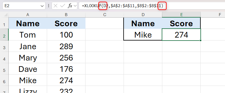
Parentheses are also used to mark the first of a function's arguments. For example, typing:
=XLOOKUP(
tells Excel that you want to perform a lookup using the XLOOKUP function, and the relevant parameters will follow the opening parenthesis. Once you've finished typing the arguments, you'll complete the formula with a closing parenthesis:
=XLOOKUP(D2,$A$2:$A$11,$B$2:$B$11)
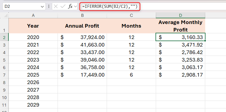
Finally, parentheses are used in Excel to nest functions. In this example, the SUM function is nested within the IFERROR function so that if the result returns an error, a blank cell is displayed:
=IFERROR(SUM(B2/C2),"")
Square Brackets: Referencing Column Headers in Tables
Square brackets are used in Excel formulas to reference a header in a formatted table.
Everything You Need to Know About Excel Tables (And Why You Should Always Use Them)
This could totally change how you work in Excel.
Let's say you've been sent this table (called Fruit_Sales), and your aim is to work out the turnover for each item in column F.
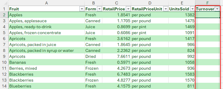
To do this, you'll need to multiply the values in column C (RetailPrice) by the values in column E (UnitsSold) for each row.
Starting in cell F2, much like when you create a formula in an unformatted dataset, type the equal (=) sign, and then click the first cell you want to include in your formula. In this case, it's cell C2.
However, notice that as soon as you click this cell, rather than adding the cell reference C2 to the formula, Excel places the column header inside square brackets—also known as a structured reference:
=[@RetailPrice]

Structured references offer several benefits in Excel. Specifically, they make formulas easier to read and understand, they save you from having to remember cell references, and they adjust dynamically to any changes you make to the table's structure or column headers.

Everything You Need to Know About Structured References in Excel
Use table and column names instead of cell references.
You'll also see that an @ symbol (also known as the intersection operator) has been added to the structured reference, which means that Excel will treat each row in this column individually, rather than adding all the values in this column together in the formula.
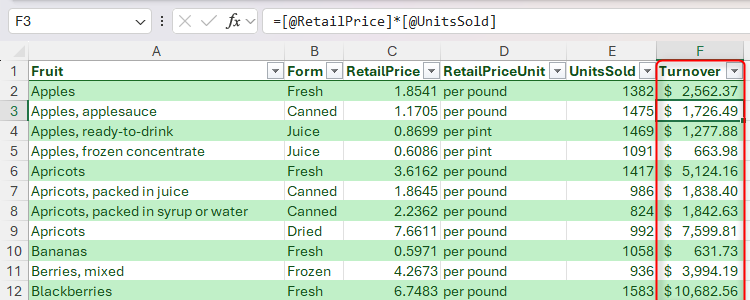
Next, add the asterisk (*) symbol to create the multiplication, and click cell E2 to insert the second argument. Again, Excel inputs a structured reference to the column header:
=[@RetailPrice]*[@UnitsSold]

When you press Enter, Excel automatically applies the formula to the remaining cells in the column, saving you the effort of doing this manually.
Structured references with square brackets don't just apply to formulas within the table itself.
For example, let's say you want to calculate the total turnover by summing all the values in column F. While you could add a total row to the bottom of the table, you prefer to have the total at the top of the spreadsheet, so that you don't have to scroll down to see it.

In this case, in cell I2, type:
=SUM(
and then hover over the column header until you see a small, black arrow. When you do, click once to select all the cells in that column of the table.

Take a moment to review the reference that has been added to the formula. Notice how, this time, the structured reference with square brackets follows the table name. This is because the formula is outside the table, so Excel needs to add an extra signpost that directs it to the correct table:
=SUM(Fruit_Sales[Turnover]
Finally, close the rounded parentheses to complete the formula, and press Enter.

Curly Braces: Defining Array Formulas and Simplifying Logical Arguments
Curly braces in Excel are primarily used to return an array, rather than a single result.
Some functions in Excel return dynamic, spilled arrays by default. For example, here, typing:
=SORT(A1:A3)
into cell C1 returns a result that starts in cell C1, and spills over to cells C2 and C3, as indicated by the blue line surrounding the cells.

However, you can also use this principle to force a function that doesn't automatically produce a dynamic array to generate more than one result.
Let's say you receive bonus payments on the 20th day of every other month, and you want to record these in a spreadsheet.
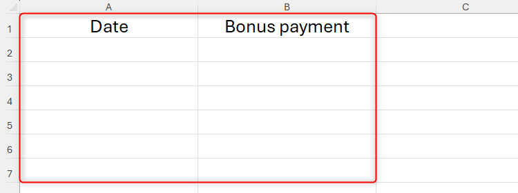
Rather than type the dates individually in column A, you can use a dynamic array formula with curly braces.
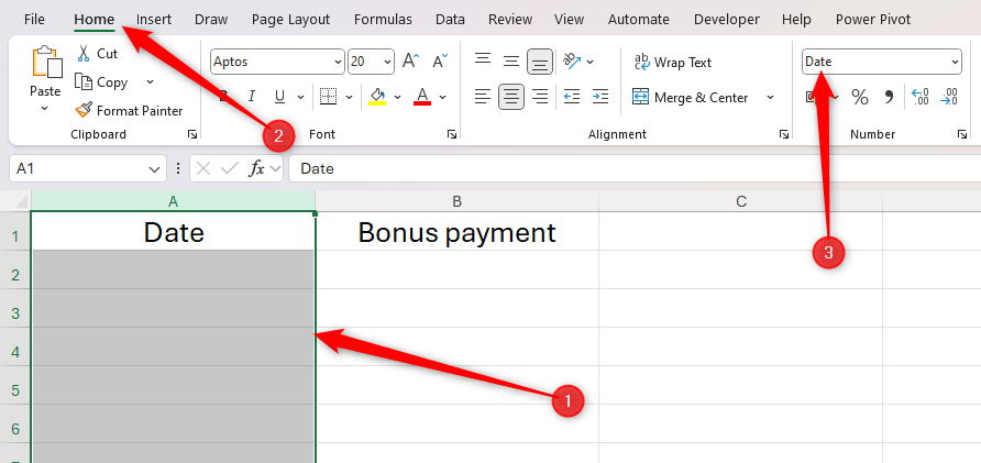
First, select column A by clicking the column header, and in the Number group of the Home tab on the ribbon, select "Date" from the drop-down list.
Excel's 12 Number Format Options and How They Affect Your Data
Adjust your cells' number formats to match their data type.
Then, in cell A2, type:
=DATE(2025,{2;4;6;8;10;12},20) where 2025 is the year, the numbers in the curly braces represent the months, and 20 is the day.
When you press Enter, Excel returns a result that spills from cell A2 to A7.
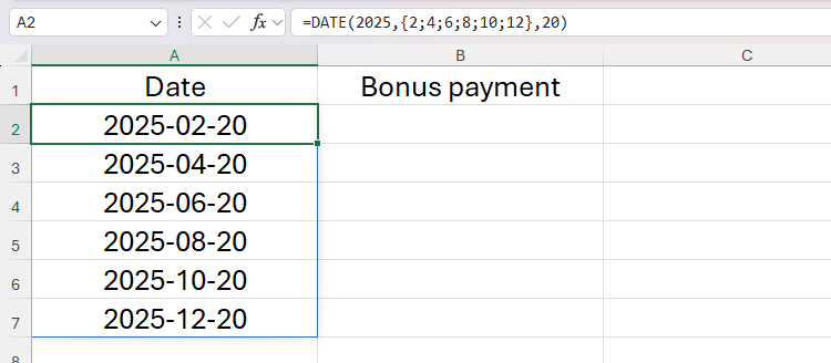
The formula containing curly braces must be placed in a cell that isn't part of a formatted Excel table. However, if the resultant values are set to remain fixed, select and copy them (Ctrl+C), and paste them as values (Ctrl+Alt+V, then V, then Enter). This converts them from a dynamic array into a regular array, meaning they can now be added to your formatted table.
On the other hand, if you want the result to spill along a row (rather than down a column), use commas (rather than semicolons) between the numbers within the curly braces. Here, typing:
=DATE(2025,{2,4,6,8,10,12},20) in cell B1 displays the dates from cell B1 to G1.

Curly braces can also be used to shorten formulas when you're using logical functions.
In this example, the IF-OR combination is used in column B to identify whether the corresponding cells in column A contain 5, 6, 7, or 8:
=IF(OR(A1=5,A1=6,A1=7,A1=8),"YES","NO")
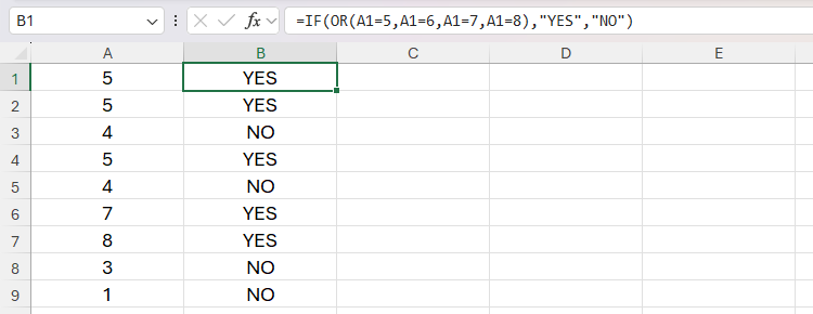
However, typing each logical argument individually can be time-consuming. Instead, enclosing the criteria within curly braces refines the logical formula and returns the same result:
=IF(OR(A1={5,6,7,8}),"YES","NO")
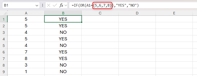
Other important symbols in Microsoft Excel formulas include the dollar ($) sign, which turns a relative reference into an absolute or mixed reference, the hash (#) sign, which acts as a spilled range operator, and the period (.), which when used in a reference to a range, trims blank cells from the result.


