There are many ways to copy and move data, duplicate forming, and link cells together in Microsoft Excel. For example, you could use Paste Special, Format Painter, or the good, old copy-and-paste combination.

However, you can execute some of these tasks much more quickly with just a couple of clicks of the mouse.

In this example, let's say you want to duplicate the values in cells A1 to C4 in cells E1 to G4. To do this, select the data, and right-click and drag the edge of the selection to the desired location.

When you release the mouse, a menu containing several useful options appears.

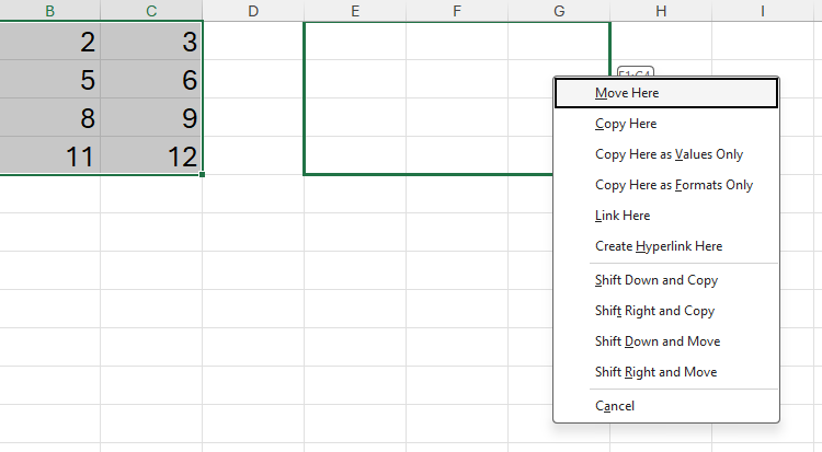
To create a copy of the source data in the destination cells, click "Copy Here." Clicking "Copy Here As Values Only" is the same as using the Paste Special tool to paste values only, and "Copy Here As Formats Only" does the same as using the Format Painter tool.

On the other hand, clicking "Link Here" generates a dynamic formula in each cell that duplicates the content of the original data, even if it changes.

The final four options in the menu allow you to shift existing data so that you can copy or duplicate the selection to the desired location. For example, clicking "Shift Down And Copy" moves any existing data that's in the way of the duplication downwards, and creates a copy of the source data in its place. Similarly, clicking "Shift Right And Move" shifts any data to the right, and moves the original data to the new location.

5 Duplicate Graphics

Right-clicking and dragging in Microsoft Excel doesn't only work with cells—it also works with graphics.

Imagine you want to duplicate the circle in this spreadsheet. To do this, right-click and drag the shape to the position where you want the copy to be.

Then, when you release the mouse, a menu appears. Click "Copy Here" to create an exact copy of the original shape.

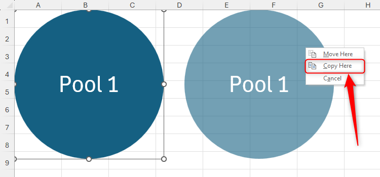
You can also use this technique with other graphics in Excel, including pictures, text boxes, and charts.

4 Filter a Dataset by the Selected Cell

One area in which Microsoft Excel truly shines is in its ability to help you visualize, read, and analyze your data. Specifically, if you want to filter your data so that only certain rows are in view, you can do so through the right-click menu.

Let's say you have this dataset, and you want to display only the products that come in canned form.

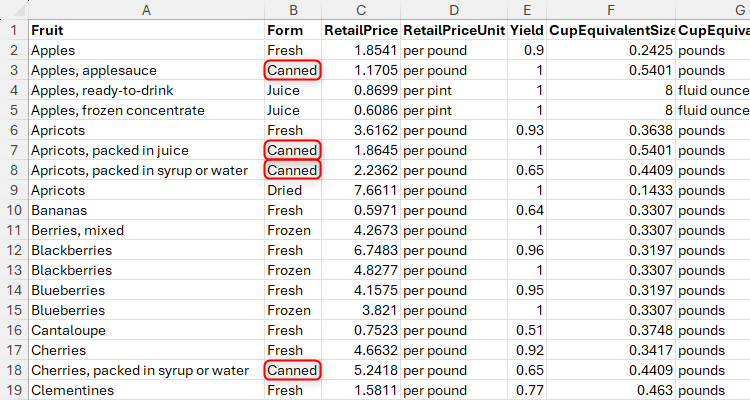
One way to achieve this would be to format the data as an Excel table, and use the filter buttons that appear by default. Alternatively, you could add filter buttons by selecting any cell in the data, and pressing Ctrl+Shift+L.

However, a quicker way to achieve the same outcome is to right-click a cell containing the word "Canned," hover over "Filter," and click "Filter By Selected Cell's Value."

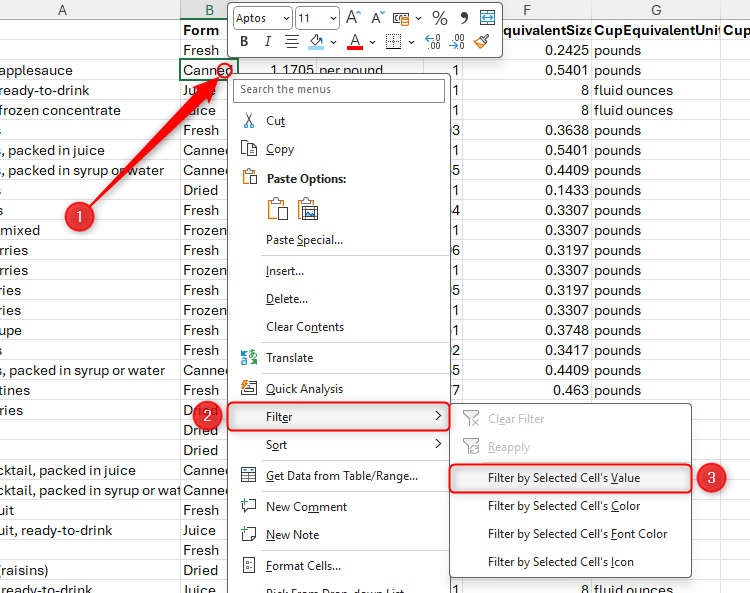
Using this method automatically adds filter buttons to the top row of the data, and displays only the rows that contain the value you selected in the previous step.

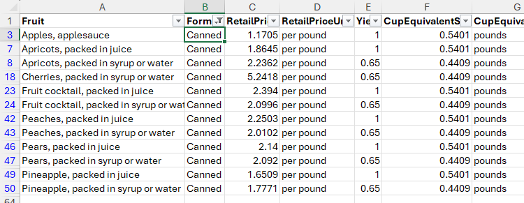
What's more, as well as filtering based on the selected cell's value, you can also choose one of the other options to filter based on the selected cell's fill color, font color, or icon. Simply choose the most appropriate option in the right-click Filter menu.

To clear the filters, select any cell in the range, and press Ctrl+Shift+L. On the other hand, to clear the filters while keeping the filter buttons, press Ctrl+Shift+L twice. Alternatively, click the relevant filter button, and click "Clear Filter From [Column Header]."

3 Pick From a Drop-Down List for Data Consistency

When adding a new row to a dataset, you can choose items from a drop-down list of existing variables.

In this example, let's say you're adding a new row headed "Watermelon."

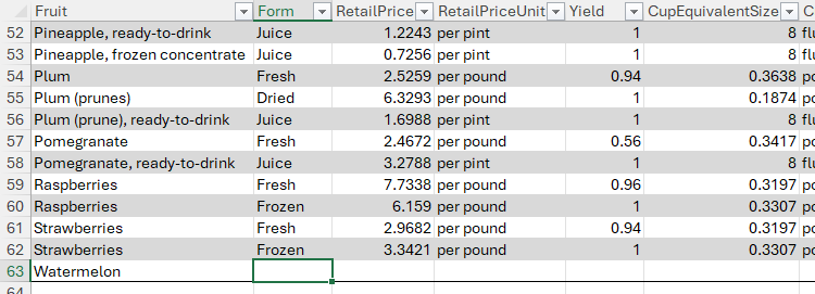
For the product form, you want to make sure that you only use one of the options that already exists in that column. To do this, right-click the cell, and select "Pick From Drop-Down List."

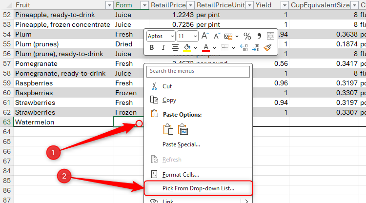
Then, a temporary list of values already inputted into this column appears. Simply click the relevant option, and Excel populates the cell with this value.

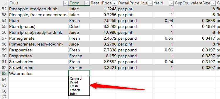
This right-click trick works best when your data is formatted as an Excel table. If it isn't, make sure there are no blank rows in the range, so that Excel recognizes each column as a continuous field.

Once you make your selection, the drop-down list disappears. The same principle can then be applied to the RetailPriceUnit column.

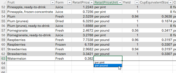
Using this method instead of typing the cell contents saves time, ensures data consistency, and helps you avoid typos.

You can also add permanent drop-down lists to cells in Excel through the Data Validation tool. This is particularly useful if you plan to add collaborators to your Excel file, and want to restrict what people can insert into a cell.

2 Search All Tools and Commands

Many people who use Microsoft Excel prefer it to its competitors due to its wider selection of powerful tools. However, this complexity means that finding the right tool among the many tabs and menus can be far too time-consuming.

One way to overcome this frustration is to right-click the cell or range of selected cells to which you want to apply a command, and type the tool in the search field at the top of the menu. As you type, the tools that match the search query appear beneath the text field.

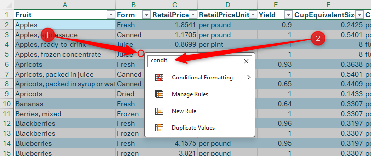
This search function doesn't return partial matches, so take care when typing the name of the tool you're searching for.

What's more, you're not limited to searching for tools. For example, if you type the name of a function and press Down Arrow > Enter, the Function Arguments dialog box appears, where you can input the relevant parameters. You can also search for and add other spreadsheet elements through this right-click search menu—like a shape, text box, or chart.

1 Navigate All Worksheets

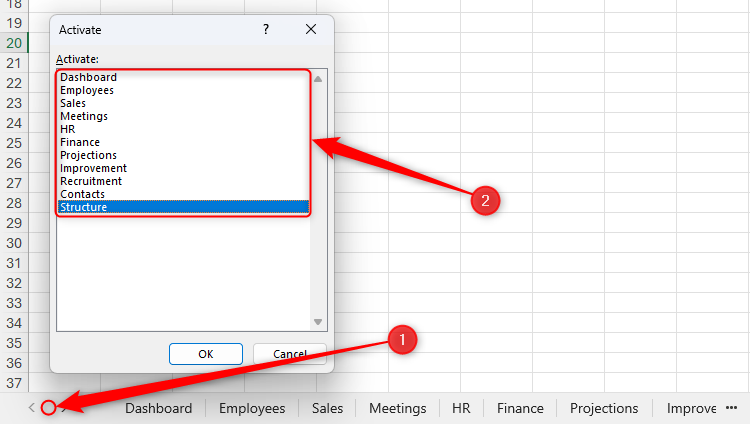
If your Excel workbook has many worksheets, navigating the horizontal tab menu at the bottom of the window can be frustrating and time-consuming.

One way to make life much easier is to right-click the arrows to the left of the tabs. This launches the Activate window, which displays all the tabs in a vertical list. As a result, you can see all the worksheet names at a glance, and simply double-click one to navigate to it.

---

Fun with your mouse in Microsoft Excel doesn't have to stop with the right-click—you can speed things up even further by learning how to use the double-click input.