Flash Fill, introduced to Microsoft Excel in 2013, was a time-saving game changer. It recognizes patterns in your data, and uses those patterns to suggest ways to automatically fill in the rest of a column.

However, despite its benefits, this tool has a severe limitation—if the source data changes, Flash Fill can't go back and reapply the pattern to the new information. In other words, the values created by Flash Fill are static, which is useless if you're trying to create a dynamic spreadsheet.

Another drawback of Flash Fill is that all the work is done behind the scenes. Yes, it can recognize patterns and complete the data for you, but you have no way of knowing how it did this. If, like me, you're interested in understanding the inner workings of your spreadsheet, this is a frustrating shortcoming.

Luckily, Microsoft recognized these issues, and came up with an excellent solution—Formula by Example.

Formula by Example: Preparing Your Data

To use Formula by Example, first, go to Excel for the Web, and log in to your Microsoft account.

Then, either open an existing spreadsheet or click "Blank Workbook" to start with a blank canvas.

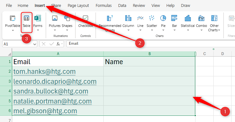
The important thing to note about Formula by Example is that it only works in formatted Excel tables, not regular ranges. So, select your data, and in the Insert tab on the ribbon, click "Table."

If your table has headers, check the box in the dialog box, and then click "OK."

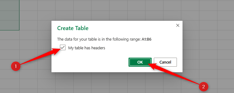
If you prefer using keyboard shortcuts, select one of the cells in your contiguous range, and press Ctrl+A to select all the cells. Then, press Ctrl+L to launch the Create Table dialog box, and finally, press Enter to create your table.

Now that you've converted your data into an Excel table in Excel for the Web, you're ready to use the Formula by Example tool.

Example 1: Transforming Text

There are many ways to transform text from one column to the next, including using the Text to Columns tool or opening Excel's Power Query Editor. However, Formula by Example is probably the most intuitive.

In this example, let's say you want to extract people's names into column B from their email addresses in column A. You also want the names to be capitalized.

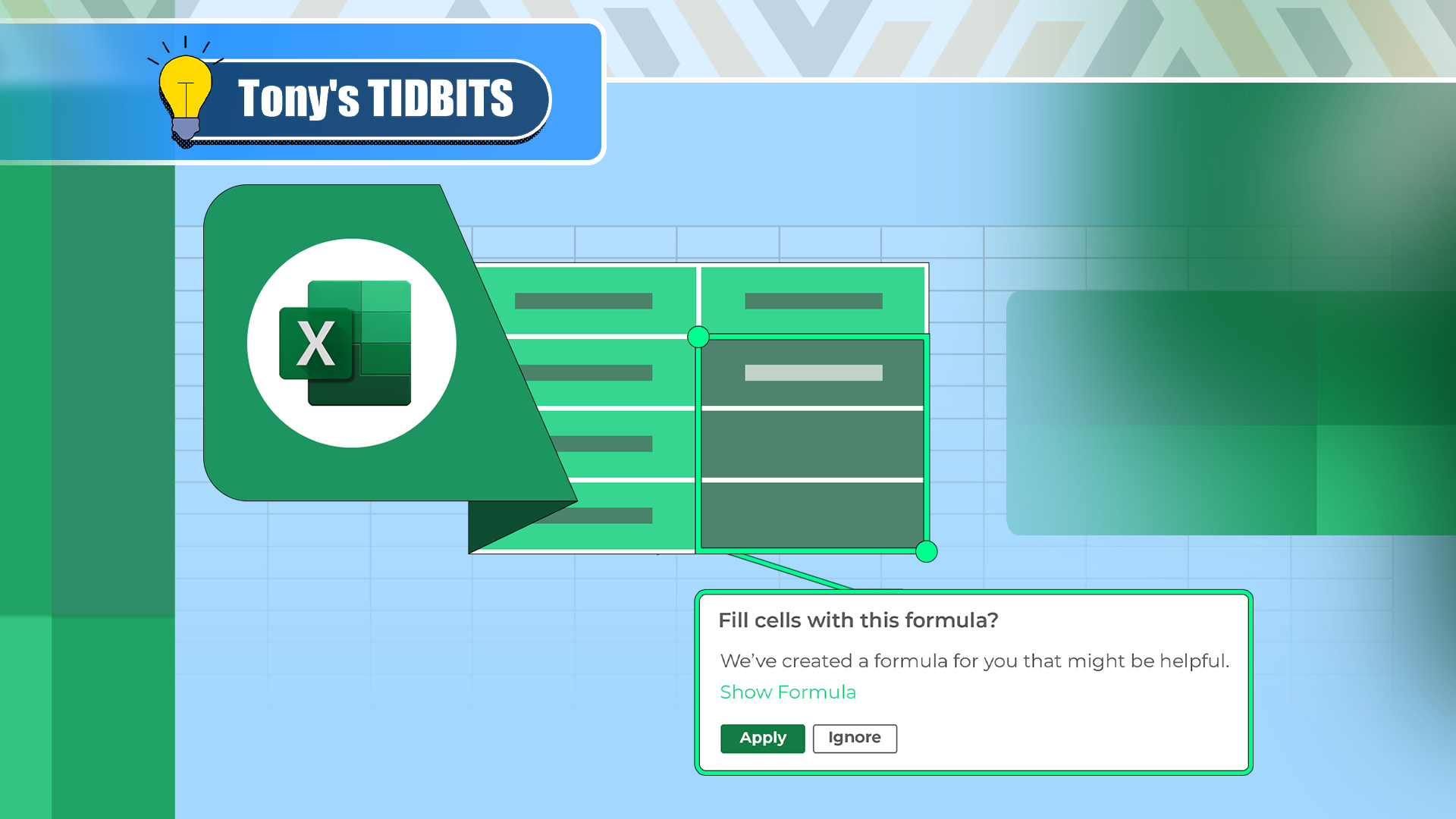
Start by typing the first couple of examples of how you want the text to be transformed. As soon as Excel recognizes a pattern, a floating window appears that offers to fill the remaining cells in that column with a formula. At this point, you can either cast your eye down the column to see whether the remaining values are as expected, or click "Show Formula" to see the formula that Excel has generated to transform the data.

In this case, the formula is:

=PROPER(TEXTBEFORE([@Email], ".", 1)) & " " & PROPER(MID(LEFT([@Email], FIND("@", [@Email]) - 1), FIND(".", [@Email]) + 1, LEN([@Email])))

where the PROPER parts of the formula deal with capitalization, and the TEXTBEFORE, MID, LEFT, FIND, and LEN parts of the formula deal with the positioning of the text to extract.

Take a moment to appreciate the complexity of this formula, and how long it might have taken you to generate it yourself. In situations like these, Formula by Example is a super handy tool that will save you lots of time.

If you're happy with what's been produced, click "Apply" to complete the column.

Now, because a formula has been used to create this text transformation, you can use it on other datasets—simply copy and paste the formula to the relevant cell, and update the parts of the formula that reference a specific column in the original table (in this case, [@Email]) with a new structured reference.

What's more, you can learn about some functions you haven't previously seen by reviewing the formula closely. Most importantly, however—and the biggest benefit of using this tool over Flash Fill—is that if the values in the precedent cells change, the formulas in the dependent cells will pick up these changes and update the result automatically.

The formula Excel generates can be specific to the structure of the original data. For example, if part of the formula looks for uppercase letters in the referenced cell, but it doesn't have any, you may see an error. To avoid this, make sure your data is consistently structured and formatted.

In a similar example, here, Excel creates a formula that extracts the first three letters of a product code into the second column of the formatted table:

=LEFT([@[Product Code]], 3)

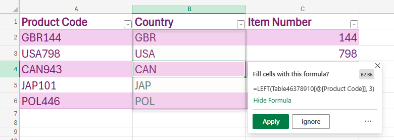
Then, I used the same principle in column C to extract the final three numbers. Here's the formula it generated:

=VALUE(RIGHT([@[Product Code]], LEN([@[Product Code]]) - 3))

Example 2: Numbering Rows

One issue with formatted Excel tables is that they're not compatible with dynamic array formulas, meaning you can't use functions that spill the result into more than one cell, like SORT or FILTER.

In this example, let's say you want to add dynamic numbers to column A so that you can keep count of the number of players in the game at any given point.

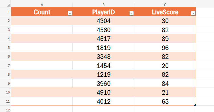
One way to do this in an unformatted area of a spreadsheet is to nest the COUNTA function within the SEQUENCE function to count the number of cells in column A that contain a value, and then use this to generate a sequence that increases by one in each row. However, this isn't possible in an Excel table, as the SEQUENCE function produces a spilled array.

However, thanks to Formula by Example, there's a workaround.

Start by typing the first few numbers into column A, and when Excel recognizes the pattern, check the formula, and click "Apply."

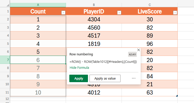
Clicking "Apply As Value" inserts the numbers as values, rather than formulas, as though you typed them manually. Essentially, Excel is giving you the option to use Flash Fill instead of Formula by Example, which, in most scenarios, isn't what you'll want to do.

Now, you know that when you add or remove rows to or from the table, the count will update automatically. What's more, you've learned that you can use the ROW function and reference the column headers to overcome the table-spill incompatibility issue I discussed earlier.

Example 3: Working With Dates

Formula by Example doesn't just help you transform text—it works just as well with dates.

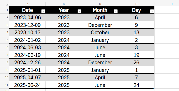
In this example, after typing the first few years into column B, Excel recognized that I was taking this information from the Date column, and produced a formula accordingly:

=YEAR([@Date])

In column C, the program saw that I was converting the month from the shorthand form to the full month name, so it generated the following formula:

=TEXT([@Date], "mmmm")

Finally, in column D, it used the DAY function to complete my dataset:

=DAY([@Date])

As with example 1, if any of the original dates in column A change, the corresponding splits in columns B, C, and D will update accordingly. Similarly, if you add more rows to the bottom of the table, they'll adopt the same formulas.

Example 4: Generating Arithmetic Calculations

Formula by Example in Excel for the Web can also work out how a result can be generated using a formula.

In this example, when I complete the first few multiplications manually, Excel spots the pattern and suggests a formula.

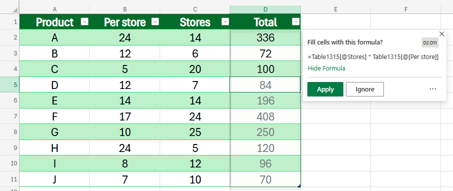
Then, in the next column, when I started rounding up the resultant values to the nearest 10, Excel recommended that I use the ROUNDUP function to complete this operation.

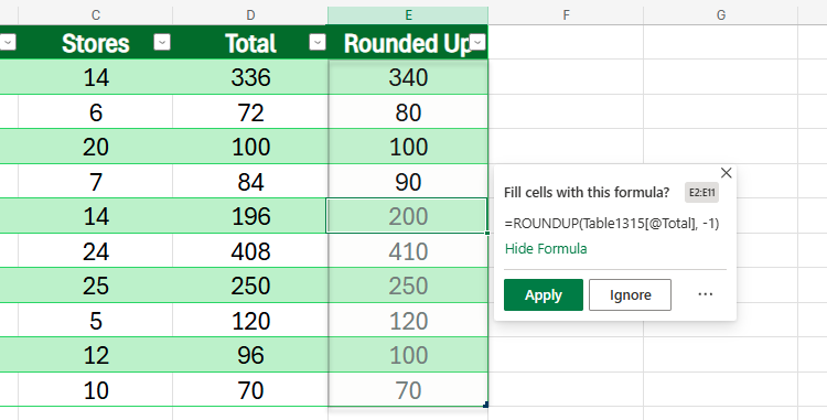
Now, let's say I made an error when inputting the number of stores in cell E3—instead of 6, it should have been 16. So, let me go back and amend that figure, and we'll see whether the values in columns D and E update automatically.

Indeed, they do, because Excel used a formula, rather than Flash Fill, to calculate these values.

---

The best way to get used to Formula by Example in Excel for the Web is to give it a go and see what it can do. For example, as well as creating formulas for the scenarios in the screenshots above, this tool can remove unnecessary spaces from your data, forward-fill a column based on examples in the first few rows, and duplicate values from a previous column while adding extra characters.