F1 is best known on Windows and Mac for being the keyboard shortcut that opens the Help document or window related to the active app. However, in Microsoft Excel, it is also a shortcut to other equally useful commands when paired with other keys.
Launch the Help Pane
If you hit a hurdle in Microsoft Excel, press F1 to bring up the Help pane, usually to the right of the window.
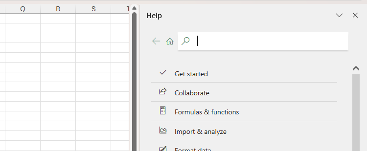
When the Help pane opens, the text field at the top is already active, so you can start typing your query straight away. As you type, suggestions will appear, and you can press Down Arrow and Enter to navigate to and select one that looks likely to help you solve your problem.
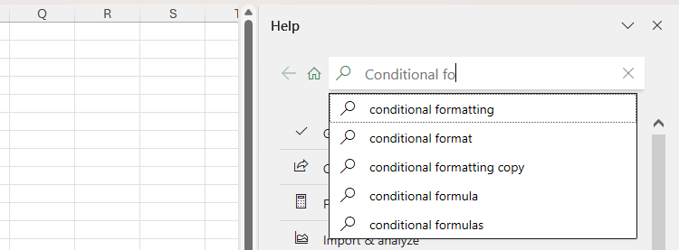
If you press F1 when you're midway through an action, the suggestions in the Help pane may relate directly to this action. This can be particularly helpful if, for example, you're using a certain function for the first time. To return to the main Help menu, with the text field still live, press Shift+Tab twice to activate the "Home" icon, then press Enter.
Alternatively, continue typing, and press Enter once you're done to see how Excel can help you.
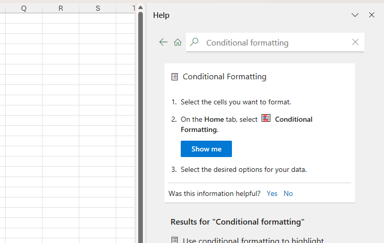
On the other hand, instead of typing a query in the text field, press Tab and Shift+Tab to navigate the suggestions, and press Enter to run the selected option.
To close the Help pane when it's still active, press Ctrl+Space, then C.

The Best Excel Keyboard Shortcuts I Use as a Power User
The key to excelling in your spreadsheet work.
Show and Hide the Ribbon
Microsoft Excel has so many tools that the ribbon takes up a large amount of real estate, especially if you're using a small screen. This limits the room you have left to work in the spreadsheet's cells.
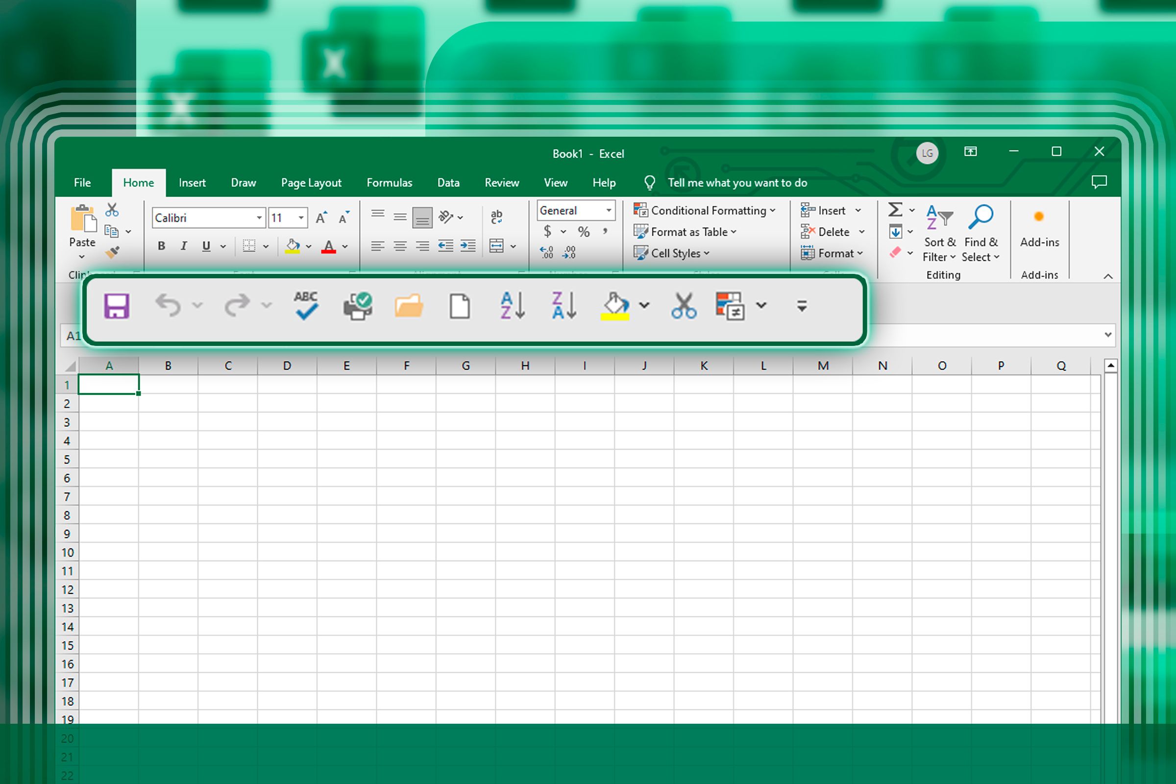
This is where Ctrl+F1 comes in handy. When you press this keyboard combo, the tool groups disappear, leaving just the name box, the formula bar, the tabs, the search field, and—if you have it activated—the Quick Access Toolbar on show above your spreadsheet.

6 Quick Access Toolbar Must-Haves in Microsoft Excel
Perform your most valuable Excel commands with a single click.
As a result, the cells occupy a larger proportion of the screen space, making data entry and analysis much easier.
To temporarily access a tab's groups, press Alt, then the letter that appears next to the relevant tab. The ribbon will disappear again if you press Esc, execute a command, or click elsewhere. Press Ctrl+F1 again to permanently show the ribbon after hiding it.
If you prefer using your mouse, you can show and hide the ribbon by double-clicking any tab.
Enter and Exit Full Screen Mode
Activating full screen mode is similar to showing and hiding the ribbon, but it goes one step further by leaving only the name box and formula bar above the worksheet, as well as the tabs below the worksheet, on display.
To enter this mode, press Ctrl+Shift+F1.

Unlike Microsoft Word, Microsoft Excel doesn't give you the option to switch to focus mode, so using full screen mode is the best way to increase your spreadsheet real estate and reduce the number of distracting icons on your screen.
Press Alt to temporarily reactivate the ribbon, or press Ctrl+Shift+F1 again to exit full screen mode.
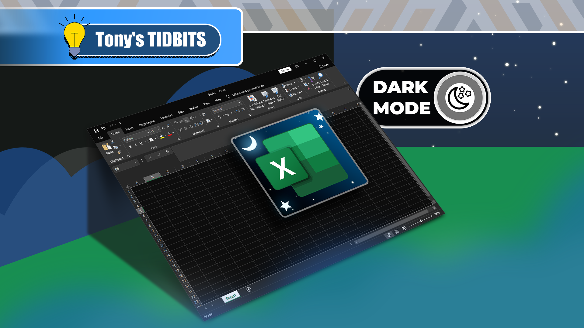
You can also switch to dark mode if you're working on your computer for an extended period and are affected by a bright screen.
Insert a Chart
Charts are a great way to quickly visualize your data in Microsoft Excel, and knowing the keyboard shortcut speeds up this process even further.
Whether your data is in an Excel table or unformatted cells, providing there are no blank rows or columns, select any cell in the range, and press Alt+F1. By default, providing your data is structured correctly, this keyboard shortcut generates a clustered column chart in the same worksheet.
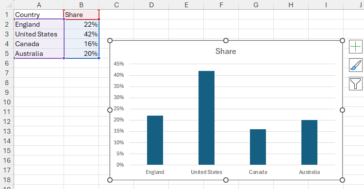
To insert the default chart on a new worksheet, press F11.
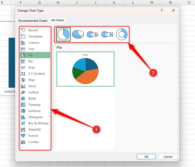
To switch this chart to another type, with the chart still selected, press Alt > JC > C to launch the Change Chart Type dialog box. There, press Tab once to activate the list of chart types (labeled 1 in the screenshot below), and use the Up and Down Arrow keys to select a chart. Next, press Tab again to activate the chart type variations (labeled 2 in the screenshot below). Finally, use the Left and Right Arrow keys to select a specific chart type, and press Enter to insert it.
The 10 Most Common Excel Charts and What They're Used For
Choose the best way to visualize your data.
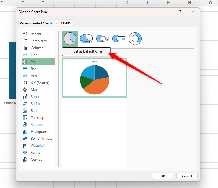
On the other hand, you can change the default chart type that is inserted whenever you press Alt+F1 in the future. To do this, follow the same process as in the step above, but rather than pressing Enter once you've landed on a chart type variation, press the menu key (also known as the application key) to launch and select the "Set As Default Chart" button. Then, press Enter to confirm.
7 of the Least-Known Excel Charts and Why You Should Use Them
They might do a better job at visualizing your data.
Add a New Worksheet
Using more than one worksheet in Excel can be a great way to organize your data. That said, having too many tabs can adversely affect your workbook's performance, so only add a new worksheet when absolutely necessary.
To add and open a new worksheet in Microsoft Excel, press Alt+Shift+F1. As you can see in the screenshot below, the tab for the new worksheet is placed to the left of the previously active worksheet tab.

If you always want new sheets to be added to the right of existing tabs, create a dummy worksheet, click and drag it so that it's the right-most tab, and always perform the Alt+Shift+F1 command from this worksheet.
Then, to rename the worksheet you just created, press Alt > H > O > R, and type the new name.

If your workbook contains more than one worksheet, press Ctrl+Page Down to move to the next worksheet or Ctrl+Page Up to move to the previous one. To delete the active worksheet, press Alt > H > D > S, but use this keyboard shortcut with caution, as you can't undo this action.
F1 isn't the only useful function key shortcut in Microsoft Excel. For example, F4 lets you toggle between reference types in formulas, repeat the last action, perform and repeat a find query, and close the active workbook or window. On the other hand, F9 is handy if you want to recalculate formulas, debug complex formulas, or minimize the Excel window.


