A dynamic array formula is a formula whose result spills over from one cell to other cells. What's more, if the result of the formula increases or decreases in size, the array does the same.

For example, typing:

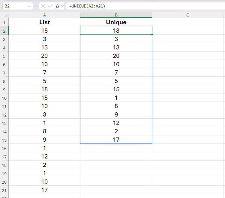
=UNIQUE(A2:A21)

into cell B2 and pressing Enter returns all the unique values from cells A2 to A21 in separate cells in column B. Notice how, when you select any of the cells containing one of those unique values, a blue line reminds you that this is a spilled array.

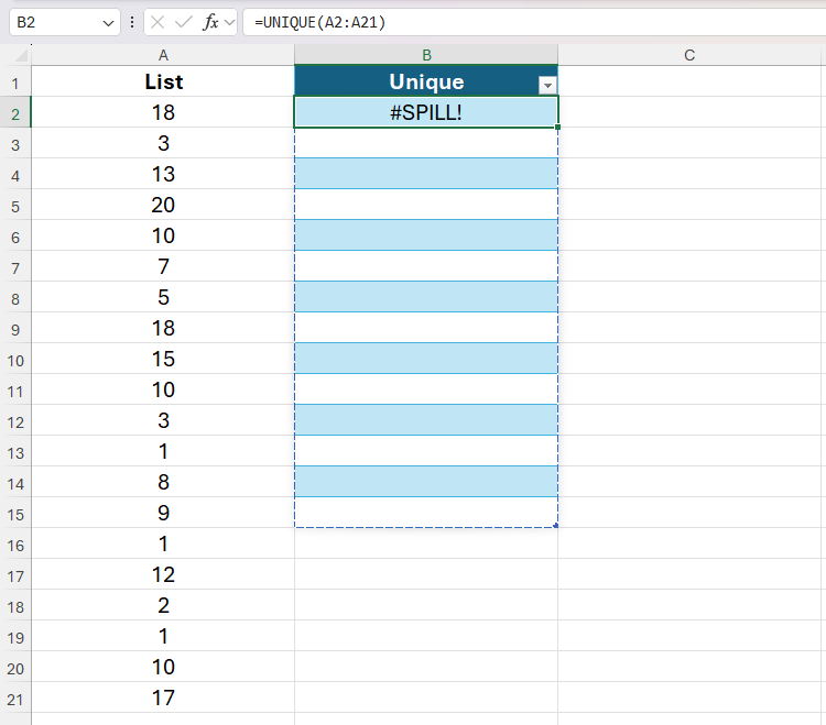
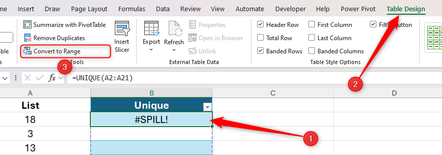
However, formatted Excel tables are designed to hold rows and columns of independent data, rather than data that spills over from a single cell. So, if you try to enter the same dynamic array formula into a cell in a table, you'll see the #SPILL! error.

Both Excel tables and dynamic array formulas are containers for automatically expanding data. So, if you try to put one thing that automatically expands (such as a dynamic array formula) inside something else that also automatically expands (such as an Excel table), Excel can't work out which of the two should dictate the size of the dataset.

In an ideal world, Microsoft would find a way to let you use dynamic array formulas within tables, with the table expanding and shrinking automatically to accommodate the spilled array. Until it does, however, I'll continue to use the following alternative approaches, which, although useful, aren't perfect fixes.

Solution 1: Convert the Table to an Unformatted Range

One way to get around this issue is to convert the Excel table to a range by selecting any cell in the table, and clicking "Convert To Range" in the Table Design tab.

Now, because the data is no longer in a structured Excel table, you can use dynamic array formulas to your heart's content.

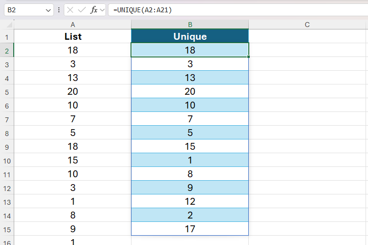
When you convert a table to a range, the formatting of the cells is retained because the conversion focuses on clearing the table's structural properties, rather than the underlying cell formatting. So, even though the range looks like a formatted table, it will behave like a regular range.

That said, even though you can reactivate the filter buttons by pressing Ctrl+Shift+L, unformatted ranges don't have the same capabilities as Excel tables. For example, you can't reference the column headers in formulas, and regular ranges don't have the same auto-expanding capacity as Excel tables.

What's more, charts and PivotTables linked to the regular data range don't automatically capture any added rows, and if you want banded rows, you'll need to apply complex conditional formatting rules.

Instead, to keep your data in a structured tabular format, you could use alternative functions that can be applied to individual rows in a table column without spilling the results.

Solution 2: Use Alternative Functions

Microsoft is always looking for ways to simplify formula-writing tasks in Excel, which is why it's introduced many swanky functions that return more than one result in recent years. However, because these don't work in tables, you could revert to some of the older functions that don't have this capability.

That said, because older functions often require more complex formulas than new, dynamic functions, they usually require more arguments and may be less efficient, especially in larger datasets.

When you type the following functions into the first row of a column in a table and press Enter, the formula will be applied to the remaining cells in that column automatically, as well as in any additional rows you subsequently add to the bottom of the table.

Generating a Dynamic Numbered List

In this example, typing:

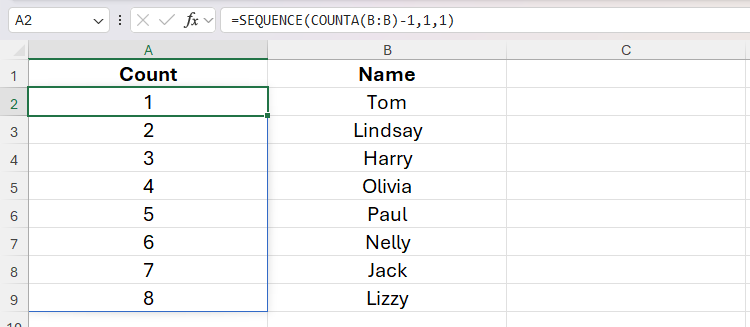
=SEQUENCE(COUNTA(B:B)-1,1,1)

into cell A2 counts the number of non-blank cells in column B, minuses one to account for the header row, and creates a single column of sequential numbers, starting at 1. What's more, if data is added to or removed from column B, the count in column A will update automatically.

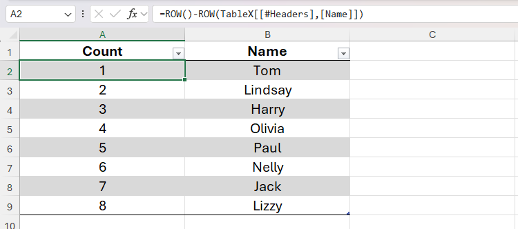
To get the same outcome in an Excel table without using a dynamic array formula, in cell A2, type:

=ROW()-ROW(TableX[[#Headers],[Name]])

Replace TableX with the correct table name and Name with the correct column name.

Creating an Array of Random Numbers

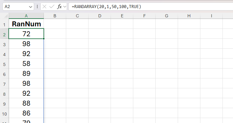
In this unformatted range, typing:

=RANDARRAY(20,1,50,100,TRUE)

into cell A2 returns a random list of whole numbers between 50 and 100 in cells A2 to A21.

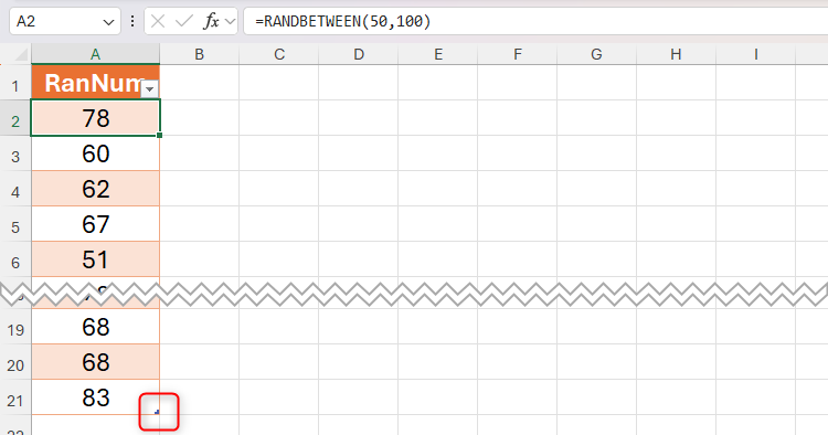
To do the same in a formatted table, in cell A2, type:

=RANDBETWEEN(50,100)

into cell A2, and click and drag the table handle to expand the table downwards until there are 20 rows of data.

RANDARRAY and RANDBETWEEN are volatile functions, meaning they recalculate each time a change is made to the worksheet. To fix the random numbers once they've been generated, select all the data (Ctrl+A), copy it (Ctrl+C), and press Crl+Shift+V to paste the numbers as values.

Splitting a Cell Into Separate Columns

In this example, TEXTSPLIT takes the name in cell A2, and spills the split version of each name into cells B2 and C2, with the comma-space string acting as the delimiter. Then, selecting cell B2 and double-clicking the fill handle applies the dynamic array formula to the remaining cells in the range.

=TEXTSPLIT(A2,", ")

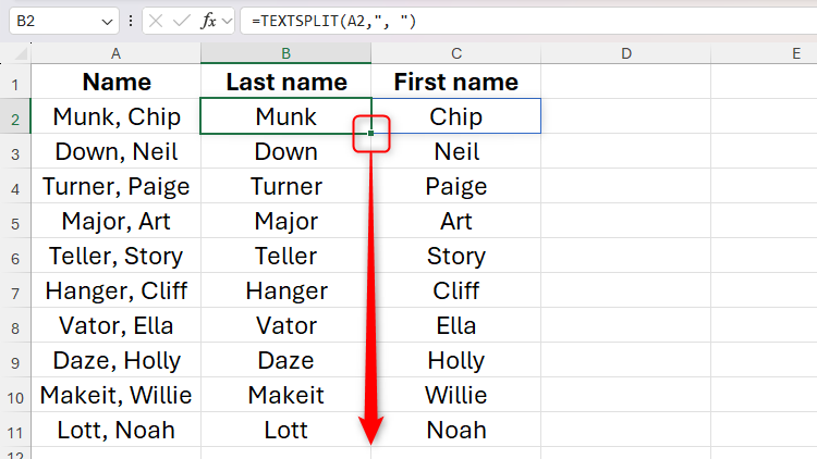
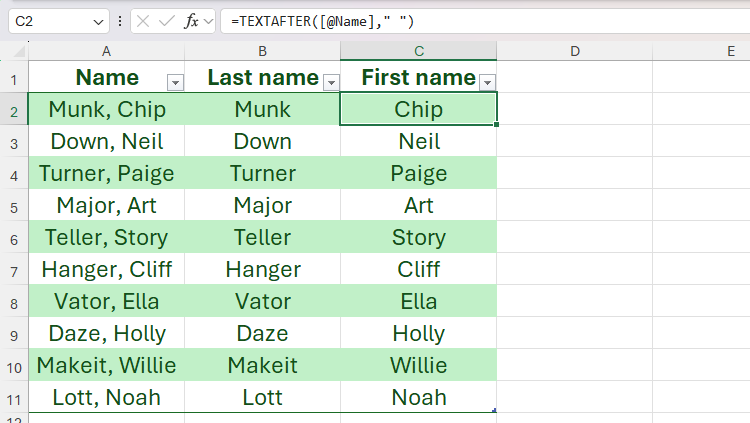
When working with Excel tables, instead of using this dynamic array formula, you can use TEXTBEFORE and TEXTAFTER.

In cell B2, type:

=TEXTBEFORE([@Name],",")

to extract the text before the comma from the Name column.

Then, in cell C2, type:

=TEXTAFTER([@Name]," ")

to extract the text after the space.

Extracting Unique Values

In this regular range, this UNIQUE formula lists all the unique values in cells A2 to A50.

=UNIQUE(A2:.A50)

Notice the period after the colon. This character, known in this context as a trim ref operator, tells Excel to trim any blank rows at the end of the result, which prevents a zero from appearing in the list.

To achieve a similar outcome in an Excel table, in cell B2, type:

=INDEX(UNIQUE($A$1:$A$50),ROW(A2))

where

• INDEX() returns a value,
• UNIQUE($A$1:$A$50), which is the first argument of the INDEX formula, finds unique values in cells A1 to A50, and
• ROW(A2), which is the second argument of the INDEX formula, returns the nth unique value, where n is the row number of the active cell.

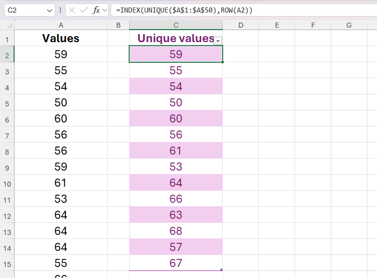
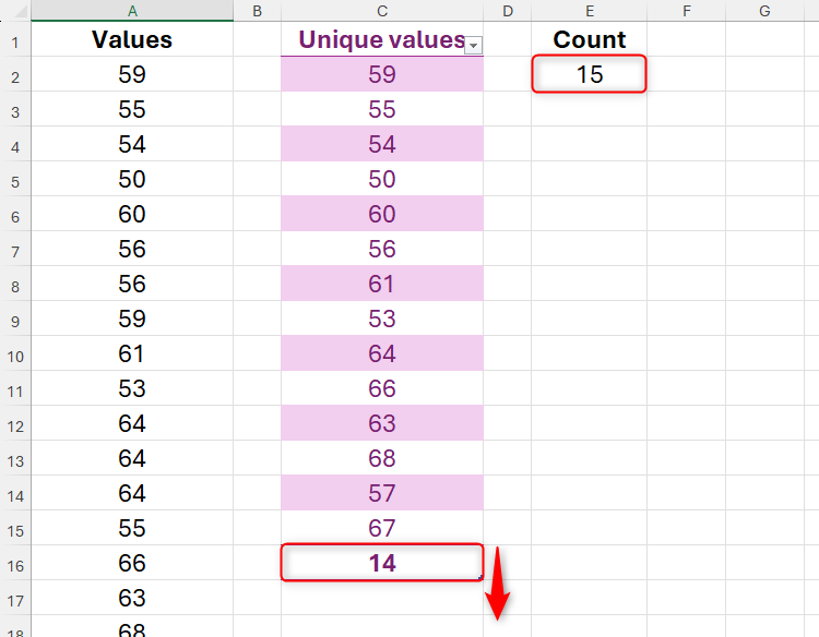
However, although this successfully finds all the unique values from the source data, the table doesn't expand and contract automatically. To account for this, in the Table Design ribbon, check "Total Row," and expand the resultant drop-down at the bottom of the table to change the aggregation type to "Count." This counts the unique values in the table column.

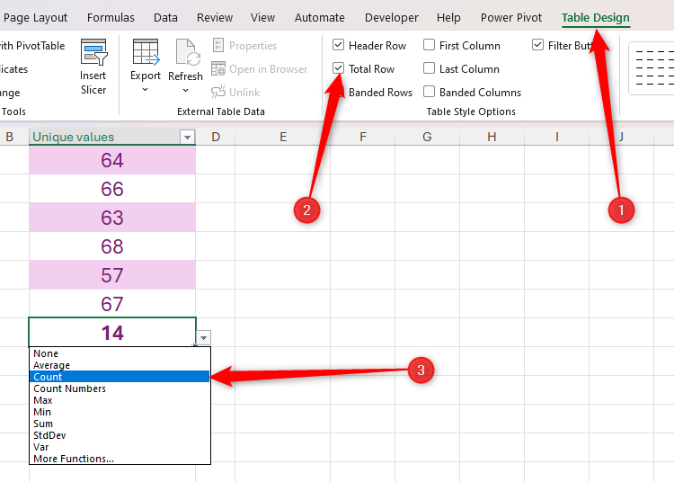
Then, in a separate cell, type:

=COUNTA(UNIQUE($A$2:.$A$50))

to count unique values in the source range.

Now, if the count in the total row of the table doesn't match the count in the COUNTA-UNIQUE cell, you know you need to expand or reduce your table size accordingly.

---

Yes, there are ways to navigate the incompatibility between Excel tables and dynamic array formulas, but admittedly, they're cumbersome and time-consuming. That's why we all need Microsoft to do us a favor and find a way to integrate these two useful tools soner rather than later.